| Issue |
Math. Model. Nat. Phenom.
Volume 15, 2020
Coronavirus: Scientific insights and societal aspects
|
|
|---|---|---|
| Article Number | 50 | |
| Number of page(s) | 14 | |
| DOI | https://doi.org/10.1051/mmnp/2020040 | |
| Published online | 11 November 2020 | |
A stochastic time-delayed model for the effectiveness of Moroccan COVID-19 deconfinement strategy*,**
1
Center for Research and Development in Mathematics and Applications (CIDMA), Department of Mathematics, University of Aveiro,
3810-193
Aveiro,
Portugal.
2
Laboratory of Analysis, Modeling and Simulation (LAMS), Faculty of Sciences Ben M’sik, Hassan II University of Casablanca,
P.B 7955 Sidi Othman,
Casablanca,
Morocco.
*** Corresponding author: This email address is being protected from spambots. You need JavaScript enabled to view it.
Received:
16
May
2020
Accepted:
28
October
2020
Abstract
Coronavirus disease 2019 (COVID-19) poses a great threat to public health and the economy worldwide. Currently, COVID-19 evolves in many countries to a second stage, characterized by the need for the liberation of the economy and relaxation of the human psychological effects. To this end, numerous countries decided to implement adequate deconfinement strategies. After the first prolongation of the established confinement, Morocco moves to the deconfinement stage on May 20, 2020. The relevant question concerns the impact on the COVID-19 propagation by considering an additional degree of realism related to stochastic noises due to the effectiveness level of the adapted measures. In this paper, we propose a delayed stochastic mathematical model to predict the epidemiological trend of COVID-19 in Morocco after the deconfinement. To ensure the well-posedness of the model, we prove the existence and uniqueness of a positive solution. Based on the large number theorem for martingales, we discuss the extinction of the disease under an appropriate threshold parameter. Moreover, numerical simulations are performed in order to test the efficiency of the deconfinement strategies chosen by the Moroccan authorities to help the policy makers and public health administration to make suitable decisions in the near future.
Mathematics Subject Classification: 60H10 / 92D30
Key words: Coronavirus disease 2019 (COVID-19) / deconfinement strategy / mathematical modeling / delayed stochastic differential equations (DSDEs) / extinction
This research is part of first author’s Ph.D. project, which is carried out at University of Aveiro.
Work partially supported through FCT, project UIDB/04106/2020 (CIDMA).
© The authors. Published by EDP Sciences, 2020
 This is an Open Access article distributed under the terms of the Creative Commons Attribution License (https://creativecommons.org/licenses/by/4.0), which permits unrestricted use, distribution, and reproduction in any medium, provided the original work is properly cited.
1 Introduction
Coronavirus disease 2019 (COVID-19), reclassified as a pandemic by the World Health Organization (WHO) on March 11, 2020 [14], is an infectious disease caused by a new type of virus belonging to the coronaviruses family and recently named severe acute respiratory syndrome coronavirus 2 (SARS-CoV-2) [4]. All the countries affected by this disease have taken many preventive measures, including containment. The containment established by the Moroccan government and the public authorities at the right time made it possible to avoid the worst: according to the minister of Health, at least 6000 lives were saved thanks to the measures adopted to face the spread of this pandemic [13]. The resistance measures, regarded as necessary and urgent, cannot be sustainable.
Actually, the deconfinement is a new stage entered by the COVID-19 pandemic. Therefore, several countries strategically planned their deconfinement strategies. The extension of the state of emergency in Morocco until May 20, 2020 will no doubt have economic repercussions. If Morocco won the first round, or at least limited the consequences, especially in terms of limiting the pandemic and health management of the situation, the second seems difficult and complex. Indeed, it must not only be well thought out but also its axes of resistance have to be well-identified. In this context, all efforts should be focused on stabilizing the economy by intelligently relying on resources. Economic deconfinement is part of the solution and should be gradual and concerted. Indeed, it is absurd to think that the return to the normality is in the near months, because the unavailability of an effective vaccine implies that the virus will always be with us in the near future, which poses a risk for the population. This economic deconfinement should be prepared and accompanied by other related measures, in particular under health, security, education and social assistance. In this period of general crisis, the response must try to mitigate the impacts on priority sectors, such as agriculture, agrifood, transport and foreign trade, in relation to imports that are vital to the Moroccan economy. The challenge is to ensure resistance and a continuity of value creation while preventing a sector from being detached from the economic body. So to speak, priority must be given to vital sectors whose health directly affects all Moroccan activity, while protecting those bordering on chaos. According to the deconfinement strategy, which is applied by the Moroccan authorities, it is mandatory to study the occurrence of an eventual second wave and it’s magnitude.
Mathematical modeling through dynamical systems plays an important role to predict the evolution of COVID-19 transmission [9, 16]. However, while taking into account the deconfinement policies, the environmental effects and the social fluctuations should not be neglected in such a mathematical study in order to describe well the dynamics and consider an additional degree of realism [2, 3, 10, 18, 21]. For these reasons, we describe here the dynamics of the deconfinement strategy by a new D-COVID-19 model, governed by delayed stochastic differential equations (DSDE), as follows:
 (1.1)
(1.1)
where S represents the susceptible sub-population, which is not infected and has not been infected before but is susceptible to develop the disease if exposed to the virus; C is the confined sub-population; Is is the symptomatic infected sub-population, which has not yet been treated, it transmits the disease, and outside of proper support it can progress to spontaneous recovery or death; Ia is the asymptomatic infected sub-population who is infected but does not transmit the disease, is not known by the health system and progresses spontaneously to recovery; Fb, Fg and Fc are the patients diagnosed, supported by the Moroccan health system and under quarantine, and subdivided into three categories: benign, severe, critical forms, respectively. Finally, R and M are the recovered and died classes, respectively. At each instant of time, the equation
![Mathematical equation: \[ D(t):=\mu_s(1-\alpha)I_s(t-\tau_3)+\mu_bF_{b}(t-\tau_4) +\mu_gF_{g}(t-\tau_4)+\mu_cF_{c}(t-\tau_4) -\sigma_3\mu_{s}I_{s}(t-\tau_3)\dfrac{\UpDelta B_3(t)}{\UpDelta t} =\dfrac{\UpDelta M(t)}{\UpDelta t} \]](/articles/mmnp/full_html/2020/01/mmnp200164/mmnp200164-eq2.png)
gives the number of the new dead due to disease. The parameter 1 − u represents the level of measures undertaken on the susceptible population while δ is the confinement rate and ρ represents the deconfinement rate. We adopt the bilinear incidence rate to describe the infection of the disease and use the parameter β to denote the transmission rate. It is reasonable to assume that the infected individuals are subdivided into individuals with symptoms and others without symptoms, for which we employ the parameter ɛ to denote the proportion for the symptomatic individuals and 1 − ɛ for the asymptomatic ones. The parameter α measures the efficiency of public health administration for hospitalization. Diagnosed symptomatic infected population is completely distributed into one of the three forms Fb, Fg and Fc, by the rates γb, γg and γc, respectively. Then, γb + γg + γc = 1. The mean recovery period of these forms are denoted by 1∕rb, 1∕rg and 1∕rc, respectively. The latter forms die also with the rates μb, μg and μc, respectively.Symptomatic infected population, which is not diagnosed, moves to the recovery compartment with a rate ηs or dies with a rate μs. On the other hand, asymptomatic infected population moves to the recovery compartment with a rate ηa. The time delays τ1 and τ2 denote the incubation period and the period of time needed before the charge by the health system, respectively. The time delays τ3 and τ4 denote the time required before the death of individuals coming from the compartments Is and the three forms Fb, Fg and Fc, respectively. Here, B1(t), B2 (t) and B3 (t) are independent standard Brownian motions defined on a complete probability space  with a filtration
  and satisfying the usual conditions, that is, they are increasing and right continuous while
  contains all P-null sets and σi represents the intensity of Bi, i = 1, 2, 3. The schematic diagram of our extended model is illustrated in Figure 1.
Remark 1.1. The stochasticity is introduced in model (1.1) by perturbing the most sensitive parameters: β, α, δ, and ρ.
Remark 1.2. For the sake of simplicity, we have assumed that the parameters δ and ρ are perturbed with the same intensities, that is, we assume that Moroccan individuals possess the same behaviors and reactions towards the authorities instructions.
Remark 1.3. Note that the multipliers of Is(t − τ2) terms are the same as σ3dB3(t) although they are premultiplied by different constants. Indeed, the portion of diagnosed symptomatic infected population is completely distributed into the three forms Fb, Fg, and Fc, by the rates γb, γg and γc, respectively. Then, γb + γg + γc = 1. In addition, we assume that the parameter α, which measures the efficiency of public health administration for hospitalization, undergoes random fluctuations.
Remark 1.4. For illustration and clarification purposes, let us suppose, as an example, that the disease progression is started from 15th of March and value of τ1 is 5. Then a susceptible individual, after contact with an infected one at instant t, becomes himself infected at instant t + τ1. Suddenly, the compartment of the infected is fed at the instant t by the susceptible infected at the instant t − τ1. Therefore, in the considered situation, when the infection starts at March 15, the term βɛ(1 − u)S(T)Is(T)∕N of new infected is equal to zero on 12th, 13th and 14th March, due to the absence of the infection.
Remark 1.5. Temporarily asymptomatic individuals are included in the class Is of symptomatic, while individuals in Ia, who are permanently asymptomatic, will remain asymptomatic until recovery and will not spread the virus, a fact which has been recently confirmed by the World Health Organization.
For biological reasons, we assume that the initial conditions of system (1.1) satisfy:
 (1.2)
(1.2)
where θ ∈ [−τ, 0] and τ = max{τ1, τ2 τ3, τ4}.
The rest of the paper is organized as follows. Section 2 deals with the existence and uniqueness of a positive global solution that ensures the well-posedness of the D-COVID-19 model (1.1). A sufficient condition for the extinction isestablished in Section 3. Then, some numerical scenarios, to assess the effectiveness of the adopted deconfinement strategy, are presented in Section 4. The paper ends up with Section 5 of conclusion.
2 Existence and uniqueness of a positive global solution
Let us denote  . We begin by proving the following result.
Theorem 2.1. For any initial value satisfying condition (1.2), there is a unique solution
![Mathematical equation: \[ x(t)=(S(t),C(t),I_s(t),I_a(t),F_b(t),F_g(t),F_c(t),R(t),M(t)) \]](/articles/mmnp/full_html/2020/01/mmnp200164/mmnp200164-eq8.png)
to the D-COVID-19 model (1.1) that remains in  with probability one.
Proof. Since the coefficients of the Stochastic Differential Equations with several delays (1.1) are locally Lipschitz continuous, it follows from [12] that for any square integrable initial value  , which is independent of the considered standard Brownian motion B, there exists a unique local solution x(t) on t ∈ [0, τe), where τe is the explosion time. For showing that this solution is global, knowing that the linear growth condition is not verified, we need to prove that τe = ∞. Let k0 > 0 be sufficiently large for
  . For each integer k ≥ k0, we define the stopping time
  , where inf ∅ = ∞.
It is evident that τk ≤ τe. Let T > 0, and define the twice differentiable function V on  as follows:
![Mathematical equation: \[ V(x):=(x_1+x_2+x_3)^2+\frac{1}{x_1}+\frac{1}{x_2}+\frac{1}{x_3}. \]](/articles/mmnp/full_html/2020/01/mmnp200164/mmnp200164-eq14.png)
By Itô’s formula, for any 0 ≤ t ≤ τk ∧ T and k ≥ 1 we have
![Mathematical equation: \[ dV(x(t))=LV(x(t))\textrm{d}t+\sigma(x(t))\textrm{d}B_t, \]](/articles/mmnp/full_html/2020/01/mmnp200164/mmnp200164-eq15.png)
where L is the differential operator of function V :
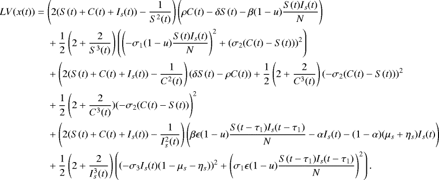
Thus,
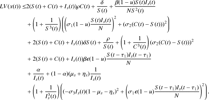
By applying the elementary inequality 2ab ≤ a2 + b2, we can easily increase the right-hand side of the previous inequality to obtain that
![Mathematical equation: \[ LV(x)\leq D(1+V(x)), \]](/articles/mmnp/full_html/2020/01/mmnp200164/mmnp200164-eq18.png)
where D is an adequate selected positive constant. By integrating both sides of the equality
![Mathematical equation: \[ dV(x(t))=LV(x(t))\textrm{d}t+\sigma(x(t))\textrm{d}B_t \]](/articles/mmnp/full_html/2020/01/mmnp200164/mmnp200164-eq19.png)
between t0 and t∧ τk and acting the expectation, which eliminates the martingale part, we get that
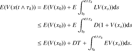
Gronwall’s inequality implies that
![Mathematical equation: \[ E(V(x(t\wedge \tau_k))\leq (EV(x_0)+DT)\exp(CT). \]](/articles/mmnp/full_html/2020/01/mmnp200164/mmnp200164-eq21.png)
For ω ∈{τk ≤ T}, xi (τk) equals k or  for some i = 1, 2, 3. Hence,
![Mathematical equation: \[ V(x_i(\tau_k))\geq \left(k^2+\frac{1}{k}\right) \wedge \left(\frac{1}{k^2}+k\right). \]](/articles/mmnp/full_html/2020/01/mmnp200164/mmnp200164-eq23.png)
It follows that

Letting k →∞, we get P(τe ≤ T) = 0. Since T is arbitrary, we obtain P(τe = ∞) = 1. With the same technique, we also deduce that the rest of the variables of the system are positive on [0, ∞). This concludes the proof.
3 Extinction of the disease
In this section, we obtain a sufficient condition for the extinction of the disease.
Theorem 3.1. Let (S(t), C(t), Is(t), Ia(t), Fb(t), Fg(t), Fc(t), R(t), M(t)) be a solution of the D-COVID-19 model (1.1) with positive initial value defined in (1.2). Assume that
![Mathematical equation: \[ \sigma_1^2> \dfrac{\beta^2}{2(\alpha+(1-\alpha)(\mu_s+\eta_s))}. \]](/articles/mmnp/full_html/2020/01/mmnp200164/mmnp200164-eq25.png)
Then,
![Mathematical equation: \[ \limsup_{t\to \infty} \ln\dfrac{I_s(t)}{t}<0. \]](/articles/mmnp/full_html/2020/01/mmnp200164/mmnp200164-eq26.png)
Namely, Is(t) tends to zero exponentially a.s., that is, the disease dies out with probability 1.
Proof. Let
![Mathematical equation: \begin{align*} d\ln I_s(t) &= \left[ \vphantom{\dfrac{1}{2I_s^{2}(t)}\left(\left(\sigma_1 \dfrac{\beta \epsilon (1-u)S(t-\tau_1)I_s(t-\tau_1)}{N} \right)^{2} + \left(\sigma_3(\mu_s+\eta_s-1)I_s(t)\right)^{2}\right)}\dfrac{1}{I_s(t)}\left(\dfrac{\beta \epsilon (1-u) S(t-\tau_1)I_s(t-\tau_1)}{N} - \alpha I_s(t) - (1-\alpha)(\mu_s+\eta_s)I_s(t)\right) \right.\\ & \quad\left. -\dfrac{1}{2I_s^{2}(t)}\left(\left(\sigma_1 \dfrac{\beta \epsilon (1-u)S(t-\tau_1)I_s(t-\tau_1)}{N} \right)^{2} + \left(\sigma_3(\mu_s+\eta_s-1)I_s(t)\right)^{2}\right)\right] \textrm{d}t\\ &\quad+ \dfrac{1}{I_s(t)} \sigma_1 \dfrac{\beta \epsilon (1-u)S(t-\tau_1) I_s(t-\tau_1)}{N} \textrm{d}B_1 + \dfrac{1}{I_s(t)} \sigma_3 (\mu_s+\eta_s-1)I_s(t) \textrm{d}B_3. \end{align*}](/articles/mmnp/full_html/2020/01/mmnp200164/mmnp200164-eq27.png)
To simplify, we set
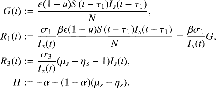
We then get
![Mathematical equation: \begin{align*} \textrm{d}\ln I_s(t) &= \dfrac{\beta G(t)}{I_s(t)} - H(t) -\dfrac{1}{2} \left(\left( \dfrac{\sigma_1 G(t)}{I_s(t)} \right)^{2}+ \left(\sigma_3(\mu_s +\eta_s-1)I_s(t)\right)^{2}\right)+ R_1(t) \textrm{d}B_{1} + R_3(t) \textrm{d}B_{3}\\ &= -\dfrac{\sigma_1^{2}}{2}\left[ \left( \dfrac{G(t)}{I_s(t)}\right) ^{2}- \dfrac{2\beta}{\sigma_1^{2}} \dfrac{G(t)}{I_s(t)}\right] + H + R_1(t) \textrm{d}B_{1}+ R_3(t) \textrm{d}B_{3}\\ &= -\dfrac{\sigma_1^{2}}{2} \left[ \left(\dfrac{G(t)}{I_s(t)} - \dfrac{\beta}{\sigma_1^{2}} \right) ^{2} - \dfrac{\beta^{2}}{\sigma_1^4} \right] + H + R_1(t) \textrm{d}B_{1} + R_3(t) \textrm{d}B_{3}\\ &\leq \,\dfrac{\beta^{2}}{2\sigma_1^{2}} + H + R_1(t) \textrm{d}B_{1} + R_3(t) \textrm{d}B_{3}. \end{align*}](/articles/mmnp/full_html/2020/01/mmnp200164/mmnp200164-eq29.png)
Hence,
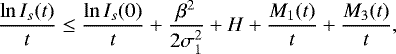
where
![Mathematical equation: \[ M_1(t)= \int_{0}^{t}R_{1}(s)\textrm{d}B_{1}, \quad M_3(t)= \int_{0}^{t}R_{3}(s)\textrm{d}B_{3}. \]](/articles/mmnp/full_html/2020/01/mmnp200164/mmnp200164-eq31.png)
We have
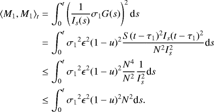
Then,
![Mathematical equation: \[ \underset{t\rightarrow\infty}{\limsup}\dfrac{\langle M_1,M_1\rangle_t}{t} \leq {\sigma_1}^2\epsilon^2(1-u)^2N^2<\infty. \]](/articles/mmnp/full_html/2020/01/mmnp200164/mmnp200164-eq33.png)
From the large number theorem for martingales [5], we deduce that
![Mathematical equation: \[ \underset{t\rightarrow\infty}{\lim}\frac{M_1(t)}{t}=0. \]](/articles/mmnp/full_html/2020/01/mmnp200164/mmnp200164-eq34.png)
We also have
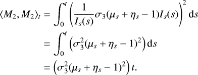
Thus,
![Mathematical equation: \[ \underset{t\rightarrow\infty}{\limsup}\dfrac{\langle M_2,M_2\rangle_t}{t} \leq \sigma^2_3(\mu_s+\eta_s-1)<\infty. \]](/articles/mmnp/full_html/2020/01/mmnp200164/mmnp200164-eq36.png)
We deduce that
![Mathematical equation: \[ \underset{t\rightarrow\infty}{\lim}\frac{M_2(t)}{t}=0. \]](/articles/mmnp/full_html/2020/01/mmnp200164/mmnp200164-eq37.png)
Subsequently,
![Mathematical equation: \[ \underset{t\rightarrow\infty}{\limsup}\dfrac{\ln I_s(t)}{t} \leq \frac{\beta^2}{2\sigma_1^2}-\alpha-(1-\alpha)(\mu_s+\eta_s). \]](/articles/mmnp/full_html/2020/01/mmnp200164/mmnp200164-eq38.png)
We conclude that if 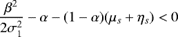 , then
  . The proof is complete.
4 Results and discussion
In this section, we simulate the forecasts of the D-COVID-19 model (1.1), relating the deconfinement strategy adopted by Moroccan authorities with two scenarios. We assume u defined as follows:
![Mathematical equation: \[ u=\left\{ \begin{array}{ll} u_{0}, & \hbox{$ \text{on}\, [\text{March 2},\text{March 10]}$;} \\ u_{1}, & \hbox{$ \text{on}\, (\text{March 10},\text{March 16]}$;}\\ u_{2}, & \hbox{$ \text{on}\, (\text{March 16},\text{March 20]}$;}\\ u_{3}, & \hbox{$ \text{on}\, (\text{March 20},\text{April 6]}$;}\\ u_{4}, & \hbox{$ \text{on}\, (\text{April 6},\text{April 25]}$;}\\ u_{5}, & \hbox{$ \text{from}\, \text{April 25} \text{ on}$;}\\ \end{array} \right. \]](/articles/mmnp/full_html/2020/01/mmnp200164/mmnp200164-eq41.png)
where ui ∈ (0, 1], for i = 0, 1, 2, 3, 4, 5, measures the effectiveness of applying the multiple preventive interventions imposed by the authorities and presented in Table 1.
COVID-19 is known as a highly contagious disease and its transmission rate, β, varies from country to country, according to the density of the country and movements of its population. Ozair et al. [17] assumed β to be [0.198 − 0.594] per day for Romania, and [0.097 − 0.291] per day for Pakistan. Further, Kuniya [10] estimated β as 0.26 (95%CI, 2.4 − 2.8). Observing the number of daily reported cases of COVID-19 in Morocco, we estimate β as 0.4517 (95%CI, 0.4484 − 0.455). After the infection, the patient remains in a latent period for 5.5 days [1, 20], in average, before becoming symptomatic and infectious or asymptomatic with a percentage that varies from 20.6% of infected population to 39.9% [15], while the time needed before his hospitalization is estimated to be 7.5 days [6, 8, 19]. All the parameter values chosen for the D-COVID-19 model (1.1) are summarized in Table 2.
Remark 4.1. From a biological point of view, the latency period is independent of the region or country under study, depending only on the structural nature of the SARS-CoV-2 coronavirus.
We consider that all measures and the adopted confinement strategy previously discussed are conserved. The evolution on the number of diagnosed infected positive individuals given by the D-COVID-19 model (1.1) versus the daily reported confirmed cases of COVID-19 in Morocco, from March 2 to May 6, is presented in Figure 2. We see that the curve generated by the D-COVID-19 model (1.1) follows the trend of the daily reported cases in Morocco. So, we confirm that the implemented measures taken by the authorities have an explicit impact on the propagation of the virus in the population since the curve of the D-COVID-19 model (1.1) has been flattening from April 17 and tends to go towards the extinction of the disease from May 05. In Figure 3, we see that Morocco has spent almost 40% of the total duration of the epidemic at May 11 and will reach extinction after four months, in average, from the start of the epidemic on March 2, 2020 (t = 0).
To prove the biological importance of delay parameters, we give the graphical results of Figure 4, which allow to compare the evolution of diagnosed positive cases with and without delays. We observe in Figure 4 a high impact of delays on the number of diagnosed positive cases. Indeed, the plot of model (1.1) without delays (τi = 0, i = 1, 2, 3, 4) is very far from the clinical data. Thus, we conclude that delays play an important role in the study of the dynamical behavior of COVID-19 worldwide, especially in Morocco, and allows to better understand the reality.
In Figures 5–7, we consider the deconfinement of 30% of the population returning to work from May 20, and this proportion is immediately integrated into the susceptible population. Numerical simulations are presented for three possible scenarios. In the first, we consider that the whole population highly respects the majority of the measures announced by the authorities in relation with the deconfinement (Fig. 5). The second and third scenarios show the direct impact on the curves when the population moderately respects the measures with different levels, σ2 = 0.10 and σ2 = 0.15, respectively.With the last two scenarios we observe the growth in the final number of infected, deaths, severe and critical forms, which are the most important to monitor, since the health system should not be saturated. It is also important to note the appearance of a second significant peak and the fact that the time required for extinction becomes longer, which relates to the value of σ2 (Figs. 6 and 7).
It should be mentioned that all our plots were obtained using the Matlab numerical computing environment by discretizing system (1.1) by means of the higher order method of Milstein presented in [7] and used in [11].
Summary of considered non-pharmaceutical interventions.
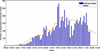 |
Figure 2 Evolution of COVID-19 confirmed cases in Morocco per day: curve predicted by our model (1.1) accordigly with Tables 1 and 2 versus real data. |
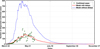 |
Figure 4 Effect of delays on the diagnosed confirmed cases versus clinical data. |
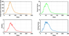 |
Figure 5 Evolution of the D-COVID-19 model (1.1) with deconfinement (ρ = 0.3) from May 20, 2020 and high effectiveness of the measures (σ2 = 0.01). |
5 Conclusion
In this work, we have proposed a delayed stochastic mathematical model to describe the dynamical spreading of COVID-19 in Morocco by considering all measures designed by authorities, such as confinement and deconfinement policies. More precisely, our model takes into account four types of delays: the first one is related to the incubation period, the second is the time needed to move from the symptomatic infected individuals to the three forms of diagnosed cases, the third is the time needed to move from the class of infected individuals to the recovered or dead class, while the last one is the time needed to pass from the three types of classes of individuals supported by the Moroccan health system, and under quarantine, to the recovered or dead compartments. Besides, to well describe reality, we have added a stochastic factor resulting from possible maladjustment of the population individuals to the measures.
To show that our model is mathematically and biologically well-posed, we have proved the global existence of a unique positive solution (see Thm. 2.1). Our result has shown a possible extinction of the disease when  is greater thana threshold parameter (see Thm. 3.1).
In addition, numerical simulations have been performed to forecast the evolution of COVID-19. More precisely, we have shown that the evolution of our D-COVID-19 model follows the tendency of daily reported confirmed cases in Morocco (see Fig. 2). Further, if Moroccan people would maintain, strictly, their confinement policy, we observe that the disease dies out around four months from March 2, 2020 (see Fig. 3). On the other hand, in response to the decision of deconfinement represented by the liberation of the 30% of population, which took place at May 20, we simulate three scenarios corresponding to different values of the intensity σ2. When σ2 = 0.01 (Fig. 5), the eradication of the disease from the population comes early compared to the cases when σ2 = 0.10 (Fig. 6) and σ2 = 0.15 (Fig. 7). Additionally, the number of diagnosed confirmed cases mainly changes because of the value of this intensity and a small perturbation leads to relevant quantitative changes and significant variations on the time needed for extinction. Thus, we observe that the value of this perturbation has a high impact on the evolution of COVID-19, which means the Moroccan population has a big interest to respect the governmental measures announced May 20, 2020, in order to have a successful and good deconfinement strategy.
Here we have compared the predictions of the proposed model (1.1) with real data until middle of May 2020. We leave the comparison of the real data in Morocco till the end of 2020 to a future work, where we also plan to incorporate the predictions of the evolution of our COVID-19 model with respect to preventive Moroccan measures by regions and cities.
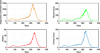 |
Figure 6 Evolution of the D-COVID-19 model (1.1) with deconfinement (ρ = 0.3) from May 20, 2020 and moderate effectiveness of the measures (σ2 = 0.10). |
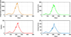 |
Figure 7 Evolution of the D-COVID-19 model (1.1) with deconfinement (ρ = 0.3) from May 20, 2020 and moderate effectiveness of the measures (σ2 = 0.15). |
Acknowledgements
The authors are grateful to an Associate Editor and two anonymous referees, who kindly reviewed an earlier version of the manuscript and provided several valuable suggestions and comments.
References
- S.G. Baum, COVID-19 incubation period: An update, Journal Watch. Available from https://www.jwatch.org/na51083/2020/03/13/covid-19incubation-period-update (2020). [Google Scholar]
- M.S. Boudrioua and A. Boudrioua, Predicting the COVID-19 epidemic in Algeria using the SIR model. Preprint medRxiv 20079467v1 (2020). [Google Scholar]
- D. Fanelli and F. Piazza, Analysis and forecast of COVID-19 spreading in China, Italy and France. Chaos Solitons Fract. 134 (2020) 109761. [CrossRef] [Google Scholar]
- A.E. Gorbalenya, S.C. Baker, R.S. Baric, R.J. de Groot, C. Drosten, A.A. Gulyaeva, B.L. Haagmans, C. Lauber, A.M. Leontovich, B.W. Neuman, D. Penzar, S. Perlman, L.L.M. Poon, D.V. Samborskiy, I.A. Sidorov, I. Sola and J. Ziebuhr, The species severe acute respiratory syndrome related coronavirus: classifying 2019-nCoV and naming it SARS-CoV-2. Nat. Microbiol. (2020) 1–9. [PubMed] [Google Scholar]
- A. Grai, D. Greenhalgh, L. Hu, X. Mao and J. Pan, A stochastic differential equations SIS epidemic model. SIAM J. Appl. Math. 71 (2011) 876–902. [Google Scholar]
- Haut Conseil de la Santé Publique, Avis relatif aux recommandations thérapeutiques dans la prise en charge du COVID-19 (complémentaire A l’avis du 5mars 2020). Available from: https://sfar.org/avis-relatif-aux-recommandations-therapeutiques-dans-la-prise-en-charge-du-covid-19/ (2020). [Google Scholar]
- D.J. Higham, An algorithmic introduction to numerical simulation of stochastic differential equations. SIAM Rev. 43 (2001) 525–546. [NASA ADS] [CrossRef] [MathSciNet] [Google Scholar]
- C. Huang, Y. Wang, X. Li, L. Ren, J. Zhao, Y. Hu, L. Zhang, G. Fan, J. Xu, X. Gu, Z. Cheng, T. Yu, J. Xia, Y. Wei, W. Wu, X. Xie, W. Yin, H. Li, M. Liu, Y. Xiao, H. Gao, L. Guo, J. Xie, G. Wang, R. Jiang, Z. Gao, Q. Jin, J. Wang and B. Cao, Clinical features of patients infectedwith 2019 novel coronavirus in Wuhan, China. Lancet 395 (2020) 497–506. [Google Scholar]
- B. Ivorra, M.R. Ferrandez, M. Vela-Perez and A.M. Ramos, Mathematical modeling of the spread of the coronavirusdisease 2019 (COVID-19) taking into account the undetected infections. The case of China. Commun. Nonlinear Sci. Numer. Simul. 88 (2020) 105303. [CrossRef] [PubMed] [Google Scholar]
- T. Kuniya, Prediction of the epidemic peak of coronavirus disease in Japan, 2020. J. Clin. Med. 9 (2020) 789. [Google Scholar]
- M. Mahrouf, K. Hattaf and N. Yousfi, Dynamics of a stochastic viral infection model with immune response. MMNP 12 (2017) 15–32. [Google Scholar]
- X. Mao, Stochastic differential equations and applications, second edition. Horwood Publishing Limited, Chichester, (2008). [CrossRef] [Google Scholar]
- Ministry of Health of Morocco, Department of Epidemiology and Disease Control. Available from: http://www.sante.gov.ma/Pages/Accueil.aspx (2020). [Google Scholar]
- Ministry of Health of Morocco, The official portal of Corona virus in Morocco. Available from: http://www.covidmaroc.ma/pages/Accueil.aspx (2020). [Google Scholar]
- K. Mizumoto, K. Kagaya, A. Zarebski and G. Chowell, Estimating the asymptomatic proportion of coronavirusdisease 2019 (COVID-19) cases on board the Diamond Princess cruise ship, Yokohama, Japan, 2020. Euro Surveill. 25 (2020) 2000180. [Google Scholar]
- F. Ndaïrou, I. Area, J.J. Nieto and D.F.M. Torres, Mathematical modeling of COVID-19 transmission dynamics with a case study of Wuhan. Chaos Solitons Fract. 135 (2020) 109846. [CrossRef] [Google Scholar]
- M. Ozair, T. Hussain, M. Hussain, A.U. Awan and D. Baleanu, Estimation of transmission potential and severity of COVID-19 in Romania and Pakistan. Preprint medRxiv 20088989v1 (2020). [Google Scholar]
- B. Tang, X. Wang, Q. Li, N. L. Bragazzi, S. Tang, Y. Xiao and J. Wu, Estimation of the transmission risk of the 2019-nCoV and its implication for public health interventions. J. Clin. Med. 9 (2020) 462. [Google Scholar]
- D. Wang, B. Hu, C. Hu, F. Zhu, X. Liu, J. Zhang, B. Wang, H. Xiang, Z. Cheng, Y. Xiong, Y. Zhao, Y. Li, X. Wang and Z. Peng, Clinical characteristics of 138 hospitalized patientswith 2019 novel coronavirus-infected pneumonia in Wuhan, China. JAMA 323 (2020) 1061–1069. [Google Scholar]
- WHO, Coronavirus disease 2019 (COVID-19) Situation Report 73. Available from: https://apps.who.int/iris/handle/10665/331686 (2020). [Google Scholar]
- J.T. Wu, K. Leung and G.M. Leung, Nowcasting and forecasting the potential domestic and international spread of the 2019-nCoV outbreak originating in Wuhan, China: a modelling study. The Lancet 395 (2020) 689–697. [CrossRef] [PubMed] [Google Scholar]
All Tables
All Figures
 |
Figure 1 Schematic diagram of model (1.1). |
| In the text | |
|
Figure 2 Evolution of COVID-19 confirmed cases in Morocco per day: curve predicted by our model (1.1) accordigly with Tables 1 and 2 versus real data. |
| In the text | |
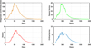 |
Figure 3 Evolution given by the D-COVID-19 model (1.1) without deconfinement (ρ = 0). |
| In the text | |
|
Figure 4 Effect of delays on the diagnosed confirmed cases versus clinical data. |
| In the text | |
|
Figure 5 Evolution of the D-COVID-19 model (1.1) with deconfinement (ρ = 0.3) from May 20, 2020 and high effectiveness of the measures (σ2 = 0.01). |
| In the text | |
|
Figure 6 Evolution of the D-COVID-19 model (1.1) with deconfinement (ρ = 0.3) from May 20, 2020 and moderate effectiveness of the measures (σ2 = 0.10). |
| In the text | |
|
Figure 7 Evolution of the D-COVID-19 model (1.1) with deconfinement (ρ = 0.3) from May 20, 2020 and moderate effectiveness of the measures (σ2 = 0.15). |
| In the text | |
Current usage metrics show cumulative count of Article Views (full-text article views including HTML views, PDF and ePub downloads, according to the available data) and Abstracts Views on Vision4Press platform.
Data correspond to usage on the plateform after 2015. The current usage metrics is available 48-96 hours after online publication and is updated daily on week days.
Initial download of the metrics may take a while.